Training and Evaluation

With the feature matrix built and preprocessed, this page covers the final step of the pipeline: splitting the data, training three classification models, and comparing their predictive performance with AUC.

Load Preprocessed Data

The preprocessing step saved the final training and test splits to CSV. Load them here:

using CSV, DataFrames
using CategoricalArrays: categorical
using MLJ

train_df = CSV.read(joinpath("output", "train.csv"), DataFrame)
test_df  = CSV.read(joinpath("output", "test.csv"),  DataFrame)

# MLJ classifiers require a CategoricalVector of strings for the target
train_df.outcome = categorical(string.(train_df.outcome); levels = ["0", "1"])
test_df.outcome  = categorical(string.(test_df.outcome);  levels = ["0", "1"])

y_train = train_df.outcome
X_train = select(train_df, Not(:outcome))

y_test  = test_df.outcome
X_test  = select(test_df,  Not(:outcome))

The levels = ["0", "1"] call ensures both the train and test vectors share the same encoding - important for models that inspect the level order internally.

Train-Test Split

The 80/20 split is performed during preprocessing (see preprocessing.jl) with a fixed random seed so the partition is reproducible:

# Done in preprocessing.jl:
# train, test = partition(df, 0.8; shuffle = true, rng = 42)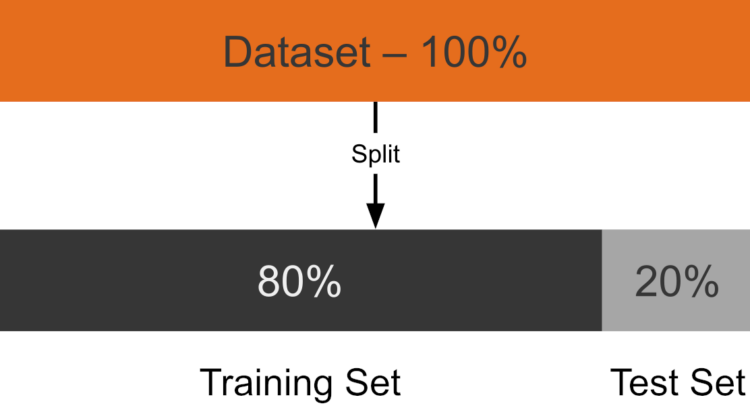

Training Models with MLJ.jl

MLJ.jl provides a uniform interface for every model family in Julia. The same machine -> fit! -> predict pattern works regardless of algorithm, making it straightforward to swap models or run comparisons.

Three models are trained and compared. The evaluation metric is AUC (Area Under the ROC Curve): 1.0 is a perfect classifier, 0.5 is random guessing.

using ROCAnalysis

function evaluate_model(model, X_train, y_train, X_test, y_test)
    mach = machine(model, X_train, y_train)
    fit!(mach; verbosity = 0)
    # pdf(..., "1") extracts the predicted probability of the positive class
    probs = pdf.(predict(mach, X_test), "1")
    score = auc(roc(probs, y_test .== "1"))
    return score, mach
end

Logistic Regression with L1 Regularization

Logistic regression is the transparent baseline. L1 regularization (Lasso) drives the coefficients of irrelevant features exactly to zero, effectively selecting the most informative predictors and keeping the model interpretable.

See: MLJLinearModels.jl documentation

using MLJLinearModels

logreg = MLJLinearModels.LogisticClassifier(penalty = :l1, lambda = 0.0428)
auc_lr, mach_lr = evaluate_model(logreg, X_train, y_train, X_test, y_test)
println("Logistic Regression  AUC: $auc_lr")

Random Forest

Random forests build an ensemble of decision trees on random subsets of the training data and average their predictions. They handle non-linear relationships naturally, require minimal preprocessing, and are robust to correlated and noisy features.

See: MLJDecisionTreeInterface.jl documentation

using MLJDecisionTreeInterface

rf = MLJDecisionTreeInterface.RandomForestClassifier(n_trees = 100, max_depth = 10)
auc_rf, mach_rf = evaluate_model(rf, X_train, y_train, X_test, y_test)
println("Random Forest AUC: $auc_rf")

n_trees = 100 provides a stable ensemble; max_depth = 10 caps each tree's complexity to reduce overfitting.

XGBoost

XGBoost (eXtreme Gradient Boosting) trains trees sequentially, with each tree correcting the residual errors of the previous one. It consistently delivers strong performance on structured tabular data and is often the best-performing algorithm in clinical prediction benchmarks.

See: MLJXGBoostInterface.jl documentation

using MLJXGBoostInterface

xgb = MLJXGBoostInterface.XGBoostClassifier(num_round = 100, max_depth = 5, eta = 0.1)
auc_xgb, mach_xgb = evaluate_model(xgb, X_train, y_train, X_test, y_test)
println("XGBoost AUC: $auc_xgb")

eta = 0.1 is the learning rate - how much each tree corrects the model. Lower values generalise better but need more boosting rounds. max_depth = 5 limits tree depth to control model complexity.

Full Pipeline Summary

The complete PLP workflow from raw database to evaluated model:

Step	Script	Key Package
Study initialization	setup	HealthBase.jl
Cohort download	setup	OHDSIAPI.jl
Data exploration	src/01_data_loader.jl	DuckDB.jl + PrettyTables.jl
Cohort SQL translation & execution	src/02_cohort_definition.jl	OHDSICohortExpressions.jl + FunSQL.jl
Feature extraction	src/03_feature_extraction.jl	DuckDB.jl + DataFrames.jl
Distribution check	src/04_distribution_check.jl	Statistics
Outcome labeling	src/05_outcome_attach.jl	DataFrames.jl
Imputation, standardization, encoding	src/06_preprocessing.jl	CategoricalArrays.jl + Statistics
Train / test split	src/06_preprocessing.jl	MLJ.jl
Model training & evaluation	src/07_train_model.jl	MLJLinearModels · MLJDecisionTreeInterface · MLJXGBoostInterface
AUC scoring	src/07_train_model.jl	ROCAnalysis.jl

The entire workflow is orchestrated by run.jl:

# run.jl
steps = [
    ("Defining cohorts",     joinpath("src", "02_cohort_definition.jl")),
    ("Extracting features",  joinpath("src", "03_feature_extraction.jl")),
    ("Checking distributions", joinpath("src", "04_distribution_check.jl")),
    ("Attaching outcomes",   joinpath("src", "05_outcome_attach.jl")),
    ("Preprocessing",        joinpath("src", "06_preprocessing.jl")),
    ("Training models",      joinpath("src", "07_train_model.jl")),
]

for (label, path) in steps
    println("\n── $label ────")
    include(path)
end

To reproduce the full pipeline:

julia --project=. run.jl

References

• Reps, J. M., Schuemie, M. J., Suchard, M. A., Ryan, P. B., & Rijnbeek, P. R. (2018). Design and implementation of a standardized framework to generate and evaluate patient-level prediction models using observational healthcare data. Journal of the American Medical Informatics Association, 25(8), 969–975. https://doi.org/10.1093/jamia/ocy032

• OHDSI Patient-Level Prediction

• OHDSI Common Data Model

• ATLAS Demo Tool

• HealthBase.jl Documentation

• JuliaHealth on GitHub