Magnus methods

Magnus methods are RF-excitation solvers that keep each time step as a rotation. They are useful when RF, gradients, or off-resonance change during a time step: you can either use a larger for speed, or keep the same and reduce time-discretization error.

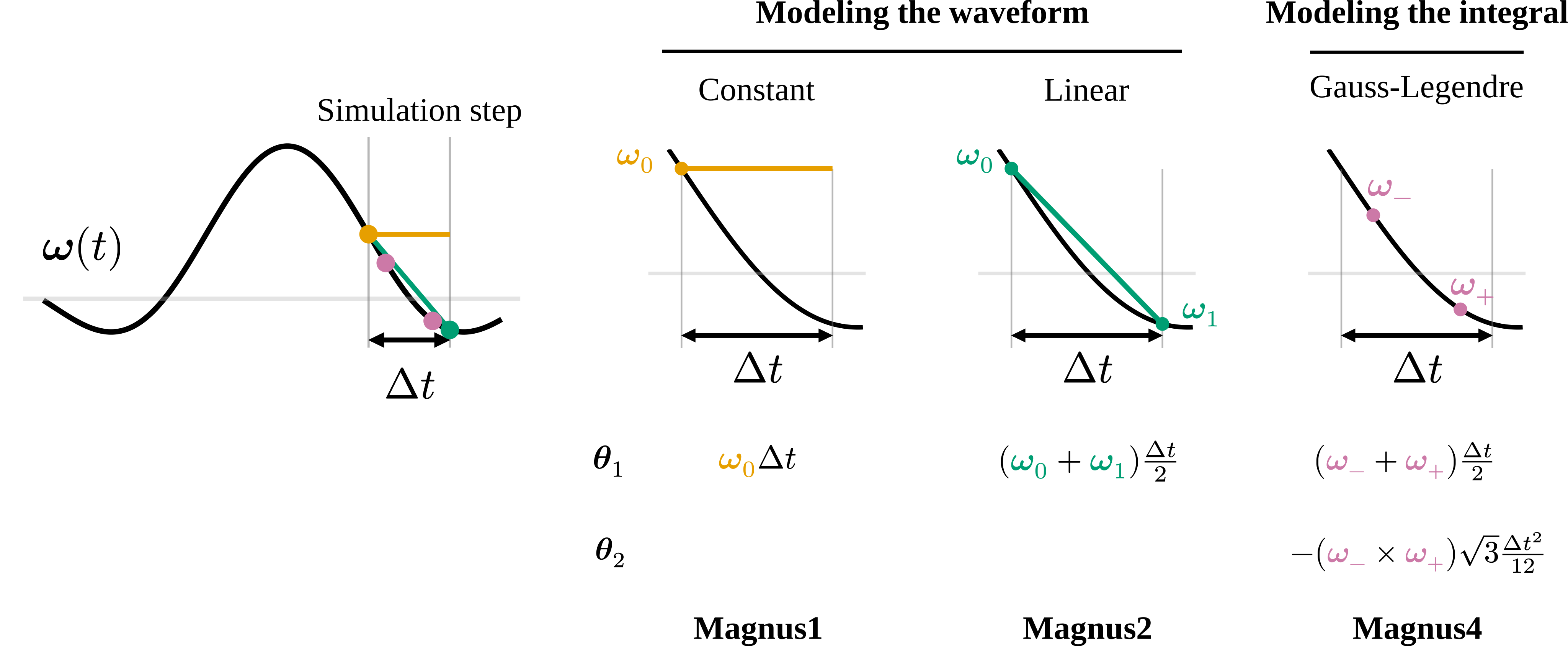
KomaMRI provides four recommended Magnus variants:

Method	Field model inside one time step	Practical use
BlochMagnus1()	piecewise constant	hard-pulse approximation / baseline
BlochMagnus2()	midpoint field	low-cost second-order default
BlochMagnus4()	Gauss-Legendre samples plus commutator correction	high accuracy, especially with Float32 GPU simulations
BlochMagnus6()	Gauss-Legendre samples plus higher-order commutators	highest smooth-order method, most useful with Float64

Use them through sim_params["sim_method"]:

sim_params = KomaMRICore.default_sim_params()
sim_params["sim_method"] = BlochMagnus2()
sim_params["Δt_rf"] = 8e-6
raw = simulate(obj, seq, sys; sim_params)

Accuracy And Step Size

The practical benefit is that higher-order Magnus methods can either improve RF excitation accuracy at the same , or reach similar accuracy with a larger .

Solid lines are Float64; dashed lines are Float32. The convergence behavior follows the expected order. In Float64, the higher-order methods keep improving as becomes smaller. In Float32, the error eventually reaches roundoff limits, so decreasing indefinitely is not always useful.

Sampling Inside A Simulation Step

A Magnus method may request additional waveform evaluations inside a simulation interval; those waveform values are combined into the rotation applied for that step.

Circles mark simulation-step boundaries. Vertical markers mark internal evaluation nodes. The node positions are normalized to one simulation interval from 0 to 1.

method   integration_nodes (0 to 1)                         intervals
Magnus1  (0,)                                                    1
Magnus2  (1//2,)                                                 2
Magnus4  (0.21132486540518713, 0.7886751345948129)               3
Magnus6  (0.1127016653792583, 1//2, 0.8872983346207417)          4

To add a new Magnus method with internal RF samples, define integration_nodes, set eval_intervals_per_step when the default interval count is not sufficient, and implement the corresponding rotation vector.

Effective Field Vector

Let be the effective field in the RF rotating frame, including RF frequency modulation. In angular-frequency units,

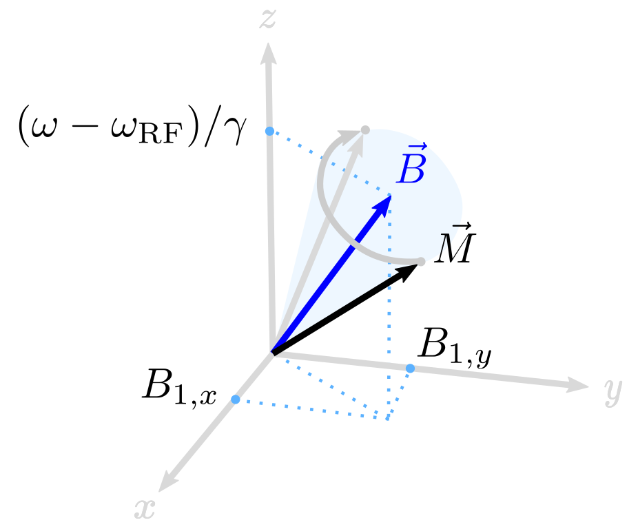
Here combines the transverse RF components and with the longitudinal frequency-offset term  .

For one excitation step, the Magnus expansion approximates the time-ordered field integral by a skew-symmetric generator:

where   is the cross-product matrix. The implementation computes directly. The Magnus rotation vector produces a rotation around with angle :

Implemented Methods

The constant, linear, and quadratic methods model inside the step.

Method	Waveform model	Magnus terms	Smooth order	Additional in-interval evaluations
BlochMagnusConst1	constant			0
BlochMagnusLin2	linear			0
BlochMagnusMid2	midpoint			1
BlochMagnusLinComm2	linear			0
BlochMagnusQuad2	quadratic			1
BlochMagnusQuad4	quadratic			1

The Gauss-Legendre methods approximate the Magnus integrals directly by evaluating at quadrature nodes.

Method	Integral approximation	Magnus terms	Smooth order	Additional in-interval evaluations
BlochMagnusGL2	Gauss-Legendre			2
BlochMagnusGL4	Gauss-Legendre			2
BlochMagnusBGL4	Blanes Gauss-Legendre			3
BlochMagnusBGL6	Blanes Gauss-Legendre			3

---

This page was generated using Literate.jl.