PLP-Pipeline Series Part 2: From Raw Clinical Data to Predictive Models

Part 2 of the PLP-Pipeline blog series – how we preprocess OMOP CDM data, extract features, and train ML models using Julia tools

Introduction 👋

Welcome back to Part 2 of the PLP-Pipeline blog series!

In Part 1, we formulated a research question, loaded synthetic patient data, and constructed our target (hypertension) and outcome (diabetes) cohorts using OHDSI definitions and Julia tools. If you haven’t read that yet, I recommend checking it out before diving in here.

Now in Part 2, we move from cohorts to models - i.e., we’ll bridge the gap between structured clinical data and predictive modeling. Specifically, we’ll walk through:

• Extracting patient-level features using cohort definitions
• Performing preprocessing (imputation, encoding, normalization)
• Splitting data into train/test sets
• Training ML models using MLJ.jl

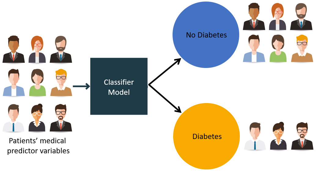
These steps will guide you through the prediction pipeline, aiming to predict the likelihood of a patient with hypertension developing diabetes.

Step 1: Feature Engineering from OMOP CDM

We extract features from several structured OMOP CDM tables such as:

Table	Features Extracted
condition_occurrence	Count of distinct parent and child conditions diagnosed or observed before the index date.
drug_exposure	Count of distinct parent and child drugs exposed, total days of drug supply, total drug quantity, and the most common drug route before the index date.
procedure_occurrence	Count of distinct past procedures undergone before the index date.
observation	Count of distinct observation concepts and the latest recorded observation value before the index date.
measurement	Maximum recorded measurement value and the most common unit of measurement before the index date.
person	Age, gender, race, and ethnicity information for the patient.

The features are computed for each patient in the target cohort using a 365-day window prior to the cohort start date.

Each table is queried independently, and the results are merged on subject_id to create a patient-level feature matrix for modeling.

Example: Drug Exposure Feature Extraction

The query below summarizes drug history for each patient using several aggregations:

• drug_count: number of distinct drug classes (using concept_ancestor for generalization)
• total_days_supply: total days covered by prescriptions
• total_quantity: total quantity of drugs supplied
• max_common_route: most frequent route of administration

File: feature_extraction.jl

# Drug exposure features: summarizing drug history in the past 365 days
drugs_query = """
SELECT 
    c.subject_id, 

    # Count of distinct parent-level drug concepts
    COUNT(DISTINCT ca.ancestor_concept_id) AS drug_count,

    # Sum of days supply to estimate treatment duration
    SUM(de.days_supply) AS total_days_supply,

    # Sum of quantity to capture volume of medication used
    SUM(de.quantity) AS total_quantity,

    # Most common route of administration
    MAX(de.route_concept_id) AS max_common_route

FROM dbt_synthea_dev.cohort c

# Join drug exposures for each subject
JOIN dbt_synthea_dev.drug_exposure de 
    ON c.subject_id = de.person_id

# Map each drug to a higher-level concept using the concept hierarchy
JOIN dbt_synthea_dev.concept_ancestor ca 
    ON de.drug_concept_id = ca.descendant_concept_id

# Filter to target cohort (e.g., patients with hypertension)
WHERE c.cohort_definition_id = 1

# Limit events to the 365 days before the cohort start date
AND de.drug_exposure_start_date BETWEEN c.cohort_start_date - INTERVAL 365 DAY AND c.cohort_start_date

# Aggregate by subject
GROUP BY c.subject_id
"""

This approach is repeated across other OMOP CDM tables (condition_occurrence, observation, measurement, procedure_occurrence, and visit_occurrence). This aligns with the paper’s recommendation to generate temporal, interpretable, and structured patient features from OMOP CDM.

Step 2: Attaching Outcome Labels

Now that we have extracted features for the target cohort (patients diagnosed with hypertension), the next step is to attach outcome labels that indicate whether a patient later developed diabetes.

We use Cohort 2 i.e outcome cohort, which includes patients from the target cohort who were subsequently diagnosed with diabetes, as defined using OHDSICohortExpressions.jl. This ensures that diabetes occurs after the hypertension event, maintaining proper temporal ordering between the target and outcome.

We query the cohort table for all subjects in outcome cohort and assign them an outcome label of 1.

File: outcome_attach.jl

diabetes_query = """
    SELECT subject_id, 1 AS outcome
    FROM dbt_synthea_dev.cohort
    WHERE cohort_definition_id = 2
"""
diabetes_df = execute(conn, diabetes_query) | > DataFrame

Next, we perform a left join with the previously created features_df, which contains covariates for all patients in the hypertension cohort. This ensures every patient has their features preserved, and only those present in the diabetes cohort will have a \(1\) under the outcome column.

For patients not found in the outcome cohort, the join results in a missing value. We treat these as negative cases \(0\), meaning the patient did not develop diabetes during the follow-up period.

df = leftjoin(features_df, diabetes_df, on=:subject_id)
df[!, :outcome] .= coalesce.(df[!, :outcome], 0)

This gives us a binary classification dataset with:

• \(1\): patient developed diabetes after hypertension
• \(0\): patient did not develop diabetes (or not within the observed period)

This labeled dataset is now ready for preprocessing and model training in later steps.

Step 3: Preprocessing for Modeling

We perform the following three tasks:

• Handling missing values
• Standardizing numeric features
• Encoding categorical variables

File: preprocessing.jl

# Impute missing values
for col in names(df)
    if eltype(df[!, col]) <: Union{Missing, Number}
        df[!, col] = coalesce.(df[!, col], 0)
    else
        df[!, col] = coalesce.(df[!, col], "unknown")
    end
end

# Standardize numerical columns
for col in [:age, :condition_count, :drug_count]
    μ, σ = mean(skipmissing(df[!, col])), std(skipmissing(df[!, col]))
    df[!, col] .= (df[!, col] .- μ) ./ σ
end

# Encode categoricals
df.gender_concept_id = categorical(df.gender_concept_id)
df.race_concept_id = categorical(df.race_concept_id)

Train-Test Splitting

Finally, we split the data into training and testing sets using an 80-20 split. This ensures we can evaluate how well the model generalizes to unseen data.

using MLJ
train, test = partition(eachindex(df.outcome), 0.8, shuffle=true)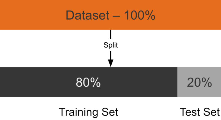

Train-Test splitting (80% - 20%)

Step 4: Model Training with MLJ.jl

We evaluated three machine learning models to identify the best-performing approach for predicting whether a patient develops diabetes. The paper specifically mentions using logistic regression (with L1 regularization) , random forest, and gradient boosting machines (like XGBoost) as part of their standardized framework.

The three models we implemented in Julia are:

• L1-Regularized Logistic Regression: Used for feature selection and classification, offering strong baseline performance and interpretability in sparse healthcare data.

• Random Forest: An ensemble method that builds multiple decision trees to capture non-linear relationships and interactions, robust against overfitting.

• XGBoost (Extreme Gradient Boosting): A boosting algorithm that sequentially builds trees to improve accuracy, known for its high predictive performance and tested in the paper for comparison.

File: train_model.jl

Shared Evaluation Function

using MLJLinearModels, MLJDecisionTreeInterface, MLJXGBoostInterface, ROCAnalysis

# Generic function to evaluate a classifier using AUC
function evaluate_model(model, X_train, y_train, X_test, y_test)
    m = machine(model, X_train, y_train)   # Bind model with data
    fit!(m)                                # Train the model
    preds = predict(m, X_test)             # Predict on test set
    probs = [pdf(p, "1") for p in preds]   # Get probability of class "1"
    auc_val = auc(roc(probs, y_test .== "1"))  # Compute AUC
    return auc_val
end

Logistic Regression

# Logistic Regression with L1 regularization
log_model = MLJLinearModels.LogisticClassifier(penalty=:l1, lambda=0.0428)
auc_log = evaluate_model(log_model, X_train, y_train, X_test, y_test)

Random Forest

# Random Forest with 100 trees
rf_model = MLJDecisionTreeInterface.RandomForestClassifier(n_trees=100)
auc_rf = evaluate_model(rf_model, X_train, y_train, X_test, y_test)

XGBoost

# XGBoost with 100 boosting rounds and depth 5
xgb_model = MLJXGBoostInterface.XGBoostClassifier(num_round=100, max_depth=5)
auc_xgb = evaluate_model(xgb_model, X_train, y_train, X_test, y_test)

Each model is trained on the same training set and evaluated on the same test set using AUC (Area Under the ROC Curve), which the paper uses as the primary metric for discrimination. This approach ensures fair comparison between models and helps identify the most suitable one for the task.

Binary Classification Model

Wrapping Up

In this post, we:

• Built patient-level features from OMOP CDM using DuckDB SQL
• Labeled outcomes based on cohort definitions
• Preprocessed the data for ML tasks
• Trained and evaluated 3 ML models using MLJ

In Part 3, I’ll wrap up with key lessons learned throughout the pipeline development - from working with real-world structured health data to implementing scalable PLP workflows in Julia. I’ll also reflect on what worked well, what could be improved, and propose directions for future enhancements. The final post will also share tips for those looking to build similar pipelines using OMOP CDM and Julia’s rich ecosystem.

Stay tuned!

Acknowledgements

Thanks to Jacob Zelko for his mentorship, clarity, and constant feedback throughout the project. I also thank the JuliaHealth community for building an ecosystem where composable science can thrive.

Jacob S. Zelko: aka, TheCedarPrince

Note: This blog post was drafted with the assistance of LLM technologies to support grammar, clarity and structure.